TL; DR
- Bayesian neural networks (BNNs) predict not only predictive results but also uncertainties, so it is an effective method to build a trustworthy AI system. However, Bayesian neural network inference is significantly slow. To tackle this problem, we proposed a novel method called vector quantized Bayesian neural network (VQ-BNN) inference that uses previously memorized predictions.
- We propose temporal smoothing of predictions with exponentially decaying importance or exponential moving average by applying VQ-BNN to data streams.
- Temporal smoothing is an easy-to-implement method that performs significantly faster than BNNs while estimating predictive results comparable to or even superior to the results of BNNs.
Translation: Korean
Recall: vector quantized Bayesian neural network improves inference speed by using previously memorized predictions
Bayesian neural networks (BNNs) predict not only predictive results but also uncertainties. However, in the previous post “Vector Quantized Bayesian Neural Network for Efficient Inference”, we raised the problem that BNNs are significantly slower than traditional neural networks or deterministic NNs. To solve this problem, we also proposed vector quantized Bayesian neural network (VQ-BNN) that improves the inference speed by using previously memorized predictions.
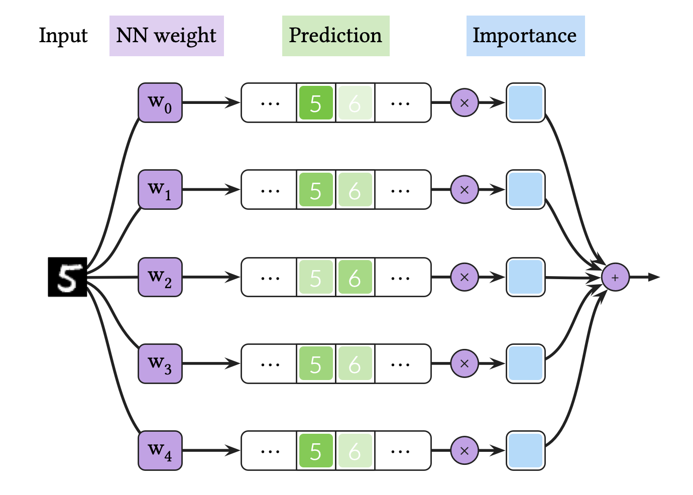
The figure above represents BNN inference. In short, BNN inference is Bayesian neural net ensemble average. BNN need iterative NN executions to predict a result for one data, and it gives raise to prohivitive comptuational cost.
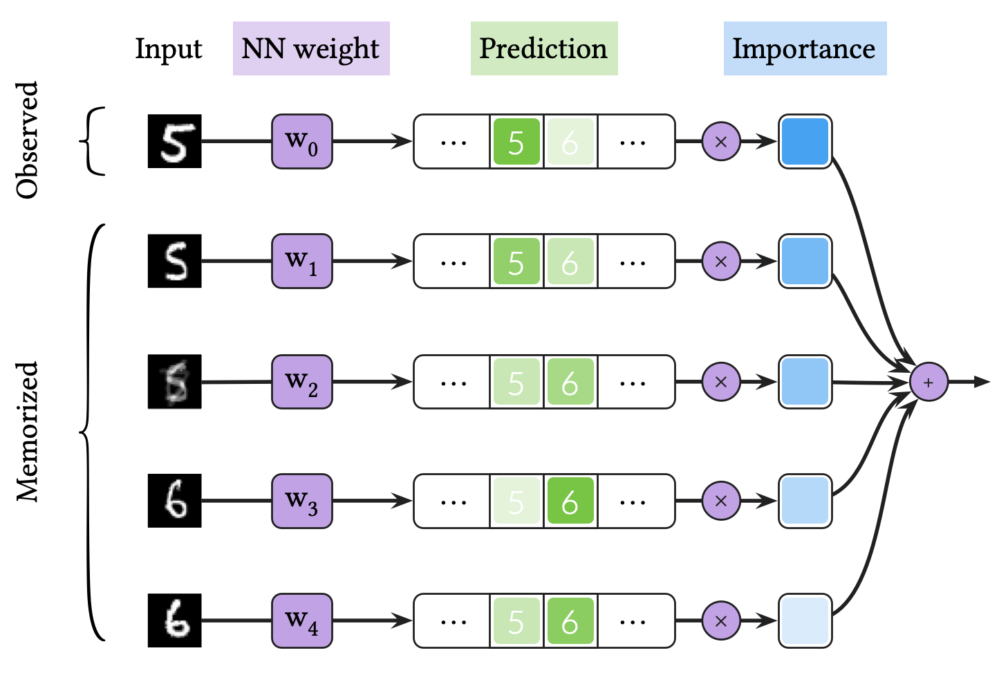
The figure above represents VQ-BNN inference. VQ-BNN inference makes a prediction for an input data only once, and compensates the predictive result with previously memorized predictions. Here, the importance is defined as the similarity between the observed and memorized data. VQ-BNN is an efficient method since it only needs one newly calculated prediction.
VQ-BNN inference needs prototype and importance. For computational efficiency, they have to meet the following requirements:
- Prototype should consist of proximate datasets.
- Importance should be easy to calculate.
Data stream analysis, especially video analysis, is an area where latency is important. Videos are large and video analysis sometimes requires real-time processing. Therefore, it is not practical to use BNN in this area because BNN inference is too slow. Instead, this post shows that VQ-BNN can process video streams easily and efficiently.
Real-world data streams are continuously chaning
In order to use VQ-BNN as the approximation theory of BNN for data streams, we exploits the property that most real-world data streams change continuously. We call it temporal consistency or temporal proximity of data streams.
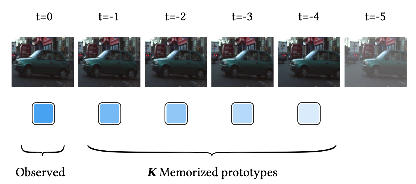
The figure above shows an example of the temporal consistency of a video sequence. In this video stream, a car is moving slowly and continuously from right to left as timestamp increases. Here, let the most recent frame be the observed input data.
Thanks to this temporal consistency, we simply take recent data as prototypes :
Similary, we propose an simple importance model which is defined as the similarity between the latest and memorized data. As shown below, it decreases exponentially over time:
where hyperparameter is decaying rate. The denominator is a normalizing constant for importance.
Taken together, VQ-BNN inference for data streams is just temporal smoothing or exponential moving average (EMA) of recent NN predictions at time :
where is a normalizing constant.
In order to calculate VQ-BNN inference, we have to determine the prediction parameterized by NN. For classification tasks, we set as a categorical distribution parameterized by the Softmax of NN logit:
where is NN logit, e.g. a prediction of NN with MC dropout layers, at time .
Temporal smoothing for semantic segmentation
We have previously shown that VQ-BNN for a data stream is a temporal smoothing of recent NN predictions. From now on, let’s apply VQ-BNN inference—i.e., temporal smoothing—to the real-world data streams. In this section, we use MC dropout as a BNN approximation.
Let’s take an example of semantic segmentation, which is a pixel-wise classification, on real-world video sequence. MC dropout predicts the Softmax (not Argmax) probability multiple times for one video frame, and averages them. It generally requires 30 samples to achieve high predictive performance, so the inference speed is decreased by 30 times accordingly.
One more thing we would like to mention is that BNN is highly dependent on input data. The input frame can be an outlier, by motion blur or video defocus or anything else. When the input frame is noisy, BNN may give an erroneous result. In this example, the window of the car is a difficult part to classify. So, most predictions of BNN are incorrect results in this case.
In contrast, VQ-BNN predicts the result for the latest frame only once, and compensates it with previously memorized predictions. It is easy to memorize the sequence of NN predictions, so the computational performance of VQ-BNN is almost the same as that of deterministic NN.
Previously, we mentioned that BNN is overly dependent on input. What about VQ-BNN? In this example, the prediction for the most recent frame is incorrect. So far, it is the same as that of BNN. However, VQ-BNN smoothen the result by using past predictions, and past predictions classify the window of the car correctly. It implies that the results of VQ-BNN are robust to the noise of data such as motion blur.
Qualitative results
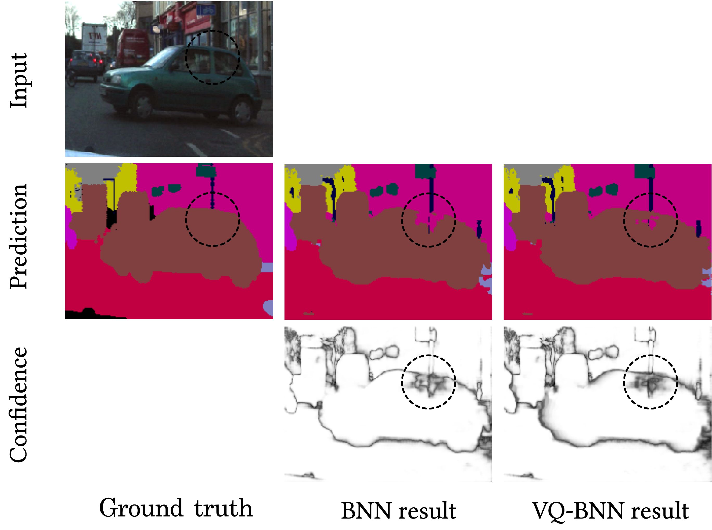
Let’s check the results. The second row shows the predictive results—i.e., Argmax of the predictive distributions—of BNN and VQ-BNN. As we expected, the result of BNN is incorrectly classified. In contrast, VQ-BNN gives a more accurate result than BNN.
The third row in this figure shows the predictive confidence—i.e., Max of the predictive distributions. The brighter the background, the higher confidence, that is the lower uncertainty. According to these confidences, VQ-BNN is less likely to be overconfident than BNN. This is because VQ-BNN uses both NN weight distribution and a data distribution at the same time.

For a better understanding, let’s compare the predictive results of each method for the above video sequence. We use vanilla deterministic neural network (DNN) and BNN (MC dropout) as baselines. And we compare them to the temporal smoothing of DNN and BNN, called VQ-DNN and VQ-BNN respectively.
These are animations of predictive results. The first column is the results of deterministic NN and BNN, and the second column is their temporal smoothings.
In these videos, the predictive results of deterministic NN and BNN are noisy. Their classification results change irregularly and randomly. This phenomenon is widely observed not only in semantic segmentation, but also in image processing using deep learning. For example, in object detection, consider a case where the size of the bounding box changes discontinuously and sometimes disappears. In contrast, temporal smoothing of deterministic NN’s and BNN’s results are stabilized. They change smoothly. So, we might get more natural results by using temporal smoothing.
Quantitative results
We previously mentioned that VQ-BNN may give a more accurate result than BNN, when the inputs are noisy. The quantitative results support the speculation.
| Method | Rel Thr (%, ↑) |
NLL (↓) |
Acc (%, ↑) |
ECE (%, ↓) |
|---|---|---|---|---|
| DNN | 100 | 0.314 | 91.1 | 4.31 |
| BNN | 2.99 | 0.276 | 91.8 | 3.71 |
| VQ-DNN | 98.2 | 0.284 | 91.2 | 3.00 |
| VQ-BNN | 92.7 | 0.253 | 92.0 | 2.24 |
This table shows the performance of the methods with semantic segmentation task on the CamVid dataset. We use arrows to indicate which direction is better.
First of all, we measure relative throughput (Rel Thr), which is the relative number of video frames processed per second. In this experiment, we use MC dropout with 30 forward passes to predict results, so the throughput of BNN is only 1/30 of that of deterministic NN. In contrast, the inference speed of VQ-BNN is comparable to that of deterministic NN, and 30✕ higher than that of BNN.
We also measure a trio for this semantic segmentation task. One is a NLL which is a proper scoring rule, two is a global pixel accuracy (Acc), and the last one is an expected calibration error (ECE) to measure the uncertainty reliability. In terms of these metrics, the predictive performance of BNN is obviously better than that of deterministic NN. More important thing is, VQ-BNN predicts more accurate results than BNN. Similarly, the results of VQ-DNN show that temporal smoothing improves predictive performance even without using BNN.
When we use deep ensemble instead of MC dropout, we obtain similar results. NLL of deep ensemble with 5 models is 0.216, and NLL of temporal smoothing with deep ensemble is 0.235 which is comparable to the result of the deep ensemble.
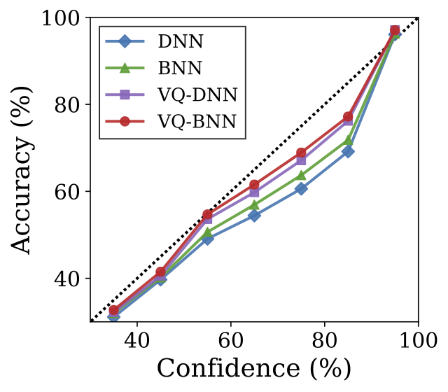
This reliability diagram also shows consistent results that temporal smoothing is an effective method to calibrate results. As shown in this figure, deterministic NN is miscalibrated. In contrast, VQ-BNN is better calibrated than deterministic NN, and surprisingly better than BNN. Likewise, VQ-DNN is better calibrated than deterministic NN and BNN.
In conclusion, using knowledge from the previous time steps is useful for improving predictive performance and estimating uncertainties. Temporal smoothing is an easy-to-implement method that significantly speeds up Bayesian NN inference without loss of accuracy.
Further reading
- This post is based on the paper “Vector Quantized Bayesian Neural Network Inference for Data Streams”. For more detailed information on VQ-BNN, please refer to the paper. For the implementation of VQ-BNN, please refer to GitHub. If you find this post or the paper useful, please consider citing the paper. Please contact me with any comments or feedback.
- For more qualitative results of semantic segmentation, please refer to GitHub.
- We have shown that predictive performance can be further improved by using future predictions—as well as past predictions. For more detailed informations, please refer to Appendix D.1 and Figure 11 in the paper.
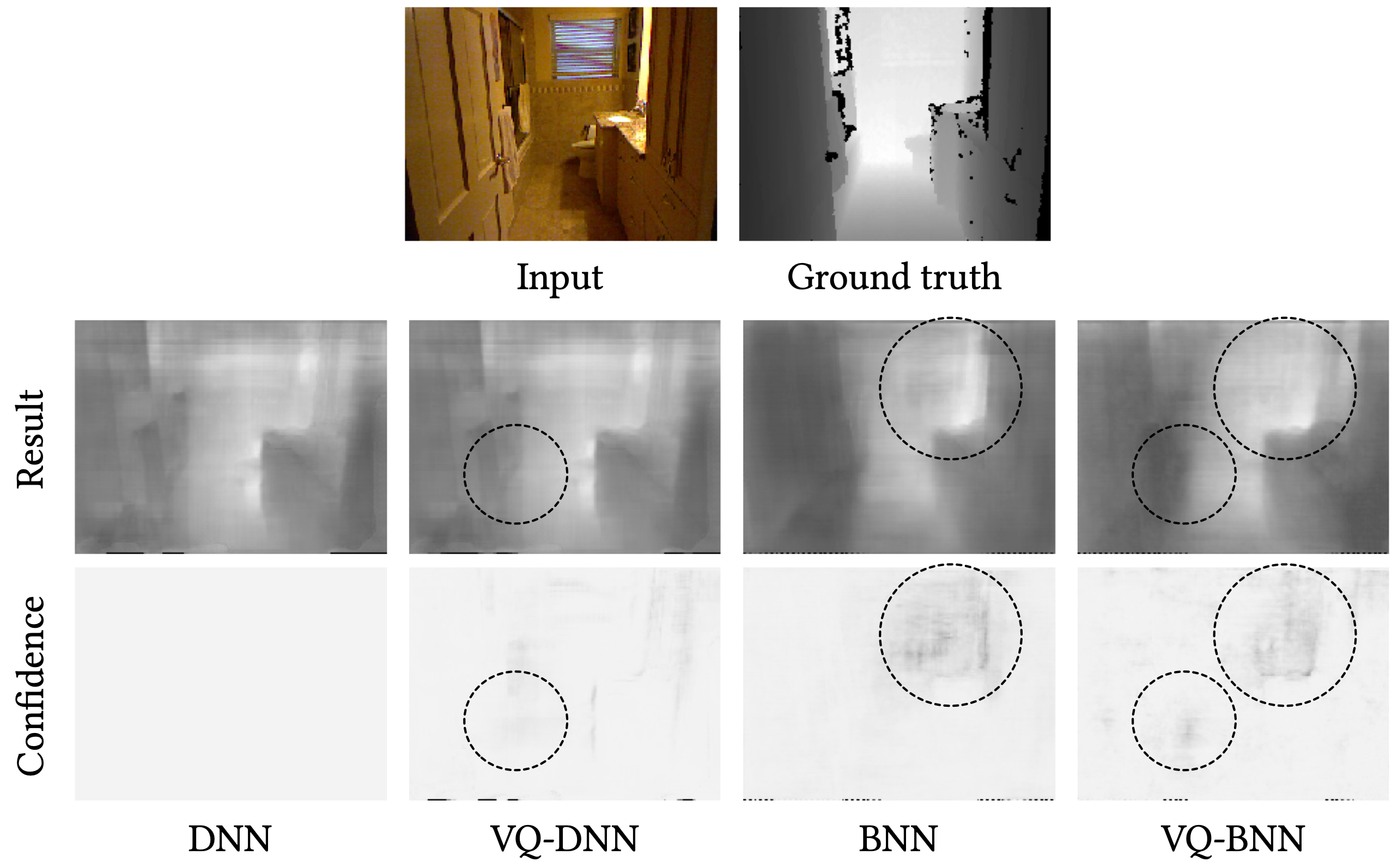
-
The figure below shows an example of the results and uncertainties for each method with monochronic depth estimation task. In this example, we observe that the uncertainty represented by VQ-DNN differs from the uncertainty represented by BNN. VQ-BNN contains both types of uncertainties. For more detailed informations, please refer to Appendix D.2 in the paper.