Vector Quantized Bayesian Neural Network for Efficient Inference

TL; DR

Bayesian neural network (BNN) is a promising method to overcome various problems with deep learning. However, BNN requires iterative neural network executions to predict a result for a single input data. Therefore, BNN inference is dozens of times slower than that of non-Bayesian neural network inference.
To tackle this problem, we propose a novel method called Vector Quantized Bayesian Neural Network. This method makes a prediction for an input data only once, and compensates the predictive result with previously memorized predictions.

Translation: Korean

Bayesian neural network estimates uncertainty and provides robustness against corrupted data

While deep learning show high accuracy in many areas, they have important problems, e.g.:

Uncertainty estimation: Deep learning cannot estimate reliable probability. For example, in a classification task, we usually interpret Softmax value of a deep learning result as a probability. However, this value is quite different from the probability that the result is correct. In practice, a confidence of the Softmax probability, i.e., Max(Softmax(nn_logit)), is higher than the true confidence. In other words, deep learning tends to predict overconfident results.
Rubustness against currupted data: Deep learning is vulnerable to adversarial attacks. In addition, the accuracy is severely compromised by natural corruptions such as weather changes, motion blur, and defocus. Moreover, shifting the input image a few pixels cause inaccurate results.

Predictions cannot be perfect and these demerits might bring about fatal consequences in some areas. For example, consider the case of autonomous driving. When an autonomous vehicle incorrectly recognize that there is nothing in front—and there are other vehicles—a collision may occur. If the autonomous driving system can predict the uncertainty, i.e. the probability that the prediction will be wrong, it will be safer and more reliable. In addition, autonomous driving systems must be safe even at night or in foggy conditions.

Bayesian deep learning, or Bayesian neural network (BNN), is one of the most promising method that can predict not only accurate results but also uncertainties. To do so, BNN uses probability distribution to model neural network (NN) weights; as opposed to traditional deep learning or deterministic neural network .

This allows computer systems to make better decisions by combining prediction with uncertainty. Also, BNN is robust to various data corruptions. In summary, BNN is an effective way to build a trustworthy AI system. In addition, BNN has various advantages such as improving prediction performance and achieving high performance in meta-learning.

However, Bayesian neural network inference is very slow

Despite these advantages, BNNs have a major disadvantage that makes it diffuclt to use as a practical tool; the predictive inference speed of BNNs is dozens of times slower than that of deterministic NNs, and the computational cost of BNNs increases dozens of times.

In this post, we are aiming to produce a fix. To do so, we must first ask why. Why is BNN inference so slow?

Brief overview of BNN inference

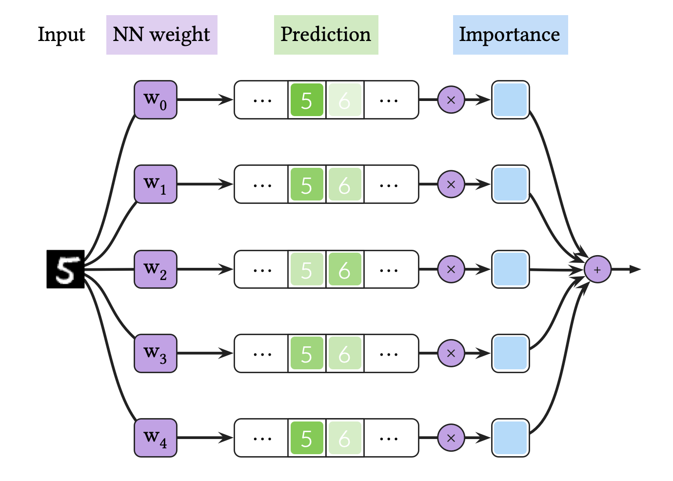
The process of BNN inference—shown in the figure above—is as follows:

Suppose that we have access to a trained NN weight probability distribution. Then, we sample NN weights from the probability and create a NN ensemble. In this figure, we create an ensemble of five NNs by using five NN weights for the toy classification task.
We use this ensemble to calculate multiple probability predictions for a single data. In this figure, we calculate five neural network logits and transform them to probabilies by using Softmax. If we use MC dropout as BNN, this process corresponds to executing multiple NN inferences for a single data, by using a NN model with dropout layers. If we use deep ensemble, it corresponds to calculating predictions for one data by using independently trained NNs.
We average the probability predictions. In this figure, we sum the probability predictions with the same importances $\frac{1}{5}$ .

So, to summarize in one sentence, BNN inference is Bayesian neural net ensemble average. Since NN execution is computationally expensive, BNN inference is five times slower than deterministic NN inference in this example. In real-world applications, BNN such as MC dropout uses 30 predictions to achieve high predictive performance, which means that the inference speed of BNN is 30✕ slower compared to deterministic NN.

Detailed explanation of BNN inference

Now, let’s move on to the details. The inference result of BNN is a posterior predictive distribution (PPD) for a single data point:

$p(\textbf{y} \vert \textbf{x}_0, \mathcal{D}) = \int p(\textbf{y} \vert \textbf{x}_0, \textbf{w}) p(\textbf{w} \vert \mathcal{D}) d\textbf{w}$

where $\textbf{x}_0$ is an observed input data, $p(\textbf{y} \vert \textbf{x}_0, \textbf{w})$ is a probability distribution parameterized by NN’s result for an input data, and $p(\textbf{w} \vert \mathcal{D})$ is a probability of trained NN weights with respect to training dataset $\mathcal{D}$ — i.e. a posterior probability in Bayesian statistics.

Unfortunately, this integral cannot be solved analytically in most cases. So, we need some approximation to calculate it. In general, we use the MC estimator as follows:

$p(\textbf{y} \vert \textbf{x}_0, \mathcal{D}) \simeq \sum_{\color{purple}{\textbf{w}_i}} \color{blue}{\frac{1}{N_{\textbf{w}}}} \color{green}{p(\textbf{y} \vert \textbf{x}_0, \textbf{w})}$

In this equation, $\color{green}{p(\textbf{y} \vert \textbf{x}_0, \textbf{w})}$ , $\color{purple}{\textbf{w}_i}$ , and blue indicates an importance. Since we write the equations in the same color as the figure, we easily compare the equation and the figure.

To approximate the predictive distribution, we use the following $N_{\textbf{w}}$ iid samples from the NN weight distribution:

$\left( \color{purple}{\textbf{w}_i}, \color{blue}{\frac{1}{N_{\textbf{w}}}} \right) \sim \color{green}{p(\textbf{w} \vert \mathcal{D})}$

This approximation says that BNN inference needs to executes NN inference $N_{\textbf{w}}$ times. As a result, the inference speed is $N_{\textbf{w}}$ times slower than deterministic NN.

How can we solve this problem? How can we calculate the neural net ensemble average in an efficient way?

Vector quantization Bayesian neural network improves inference speed by using previously memorized predictions

To tackle the problem that BNN inference is significantly slow, we propose a novel method called vector quantized Bayesian neural network (VQ-BNN). Here is the main idea: In VQ-BNN, we executes NN prediction only once, and compensate the result with previously memorized predictions.

Brief overview of VQ-BNN inference

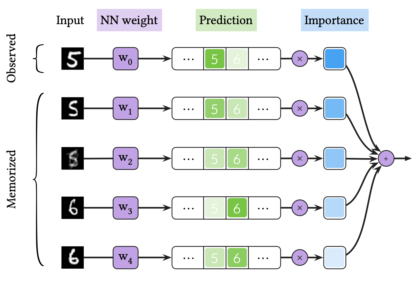
The process of VQ-BNN inference shown in the figure above is as follows:

We obtain the NN weight distribution in the same way as BNN training. We sample a NN weight from the trained NN weight distribution. Then, we make a single prediction for the observed input data with the NN weight.
Suppose that we have access to previously memorized inputs and the corresponding predictions. We calculate importances for the memorized input data. The importance is defined as the similarity between the observed and memorized data.
We averages the newly calculated prediction for observed data and memorized predictions, with importances.

In short, VQ-BNN inference is importance-weighted ensemble average of the newly calculated prediction and memorized predictions. That means, VQ-BNN compensates the result with memorized predictions for memorized inputs, also called quantized vectors or prototypes. If the time to calculate importances is negligible, it takes almost the same amoutn of time to executes VQ-BNN inference and to execute NN prediction once.

Detailed explanation of VQ-BNN inference

Let’s move on to the details. As an alternative to the predictive distribution of BNN for one data point $\textbf{x}_0$ , we propose a novel predictive distribution for a set of data $\mathcal{S}$ :

$p(\textbf{y} \vert \mathcal{S}, \mathcal{D}) = \int p(\textbf{y} \vert \textbf{x}, \textbf{w}) \, p(\textbf{x} \vert \mathcal{S}) \, p(\textbf{w} \vert \mathcal{D}) \, d\textbf{x} d\textbf{w}$

To do so, we introduce a probability distribution of data $p(\textbf{x} \vert \mathcal{S})$ . When the source is stationary, the probability represents the observation noise. For the case where the set of data $\mathcal{S}$ is from a noiseless stationary source, i.e., $p(\textbf{x} \vert \mathcal{S}) = \delta(\textbf{x} - \textbf{x}_0)$ , this predictive distribution is equal to the predictive distribution of BNN.

We can rewrite it as follows:

$p(\textbf{y} \vert \mathcal{S}, \mathcal{D}) = \int p(\textbf{y} \vert \textbf{x}, \textbf{w}) \, p(\textbf{x}, \textbf{w} \vert \mathcal{S}, \mathcal{D}) \, d\textbf{x}d\textbf{w}$

For simplicity, we introduce $p(\textbf{x}, \textbf{w} \vert \mathcal{S}, \mathcal{D}) = p(\textbf{x} \vert \mathcal{S}) \, p(\textbf{w} \vert \mathcal{D})$ . Then, we easily observe the symmetry of $\textbf{x}$ and $\textbf{w}$ .

This Equation also cannot be solved analytically, and we need an approximation as well. Here, we don’t use MC estimator which uses iid samples; instead, we approximate the equation by using importance sampling as follows:

$p(\textbf{y} \vert \mathcal{S}, \mathcal{D}) \simeq \sum_{\color{purple}{\left( \textbf{x}_{i}, \textbf{w}_{i} \right)}} \color{blue}{\pi(\textbf{x}_{i}, \textbf{w}_i \vert \mathcal{S}, \mathcal{D})} \, \color{green}{p(\textbf{y} \vert \textbf{x}_{i}, \textbf{w}_{i})}$

Here we use the following quantized vector samples and importances:

$\left( \color{purple}{(\textbf{x}_{i}, \textbf{w}_{i})}, \color{blue}{\pi(\textbf{x}_{i}, \textbf{w}_{i} \vert \mathcal{S}, \mathcal{D})} \right) \sim \color{green}{p(\textbf{x}_{i}, \textbf{w}_{i} \vert \mathcal{S}, \mathcal{D})}$

In this equation, $\color{green}{p(\textbf{y} \vert \textbf{x}_0, \textbf{w})}$ , $\color{purple}{(\textbf{x}_i, \textbf{w}_i)}$ , and $\color{blue}{\pi(\textbf{x}_{i}, \textbf{w}_i \vert \mathcal{S}, \mathcal{D})}$ . As above, it is easy to compare the equation and the figure above because the equation are written in the same color as the figure.

Why do we use the samples with different importances, instead of iid samples? This is because we try to represent the probability of $\textbf{x}$ and $\textbf{w}$ , i.e., $p(\textbf{x}_{i}, \textbf{w}_{i} \vert \mathcal{S}, \mathcal{D})$ , by changing the importance with the fixed data-weight samples. Following this perspective, we call the data-weight samples prototypes or quantized vectors.

We can improve the inference speed by using VQ-BNN. Let’s divide the predictive distribution of VQ-BNN expressed as a summation by the first term and the remainder. Without loss of generality, let $\textbf{x}_0$ be the observed data. Then, the first term of the equation $\pi(\textbf{x}, \textbf{w} \vert \mathcal{S}, \mathcal{D}) \, p(\textbf{y} \vert \textbf{x}_{0}, \textbf{w}_{0})$ refers to the prediction of the NN for observed data, which is a newly calculated prediction. And the remainder $\sum_{i = 1}^{N_{\textbf{w}}} \pi(\textbf{x}_{i}, \textbf{w}_{i} \vert \mathcal{S}, \mathcal{D}) \, p(\textbf{y} \vert \textbf{x}_{i}, \textbf{w}_{i})$ refers to the memorized NN predictions for memorized inputs and weights. If the time to calculate importances are negligible, it takes almost the same time as performing NN prediction only once.

Simplifying importance to depend only on $\textbf{x}$ (optional). The notation of the importance $\pi(\textbf{x}_{i}, \textbf{w}_{i} \vert \mathcal{S}, \mathcal{D})$ indicates that it depends not only on the data $\textbf{x}$ but also on the NN weight $\textbf{w}$ . In fact, the importance does not depend on the NN weight, i.e., $\pi(\textbf{x}_{i}, \textbf{w}_{i} \vert \mathcal{S}, \mathcal{D}) = \pi(\textbf{x}_{i} \vert \mathcal{S})$ . Therefore, we define importance using only the similarity between the data.

The reason is as follows. Let $f(\textbf{x}, \textbf{w})$ be a distribution of data and NN weight tuple sample $\{ (\textbf{x}_i, \textbf{w}_i) \}$ , i.e., $(\textbf{x}_i, \textbf{w}_i) \sim f(\textbf{x}, \textbf{w})$ . Then, we rewrite $p(\textbf{x}, \textbf{w} \vert \mathcal{S}, \mathcal{D}) = \frac{p( \textbf{x}, \textbf{w} \vert \mathcal{S}, \mathcal{D})}{f( \textbf{x}, \textbf{w})} f( \textbf{x}, \textbf{w})$ . Since $p(\textbf{x}, \textbf{w} \vert \mathcal{S}, \mathcal{D}) = \pi( \textbf{x}, \textbf{w} \vert \mathcal{S}, \mathcal{D}) f( \textbf{x}, \textbf{w})$ , we obtain $\pi( \textbf{x}, \textbf{w} \vert \mathcal{S}, \mathcal{D}) = \frac{p( \textbf{x}, \textbf{w} \vert \mathcal{S}, \mathcal{D})}{f(\textbf{x}, \textbf{w})}$ .

Suppose that $\{ \textbf{w}_i \}$ is iid NN weight samples from the posterior $p( \textbf{w} \vert \mathcal{D})$ , i.e., $\{ \textbf{w}_i \} \sim p( \textbf{w} \vert \mathcal{D})$ . Then, we can decompose $f(\textbf{x}, \textbf{w})$ into the posterior and a distribution $g(\textbf{x})$ that depends only on $\textbf{x}$ , i.e., $f(\textbf{x},\textbf{w}) = g(\textbf{x}) \, p(\textbf{w} \vert \mathcal{D})$ . By definition, $p(\textbf{x}, \textbf{w} \vert \mathcal{S}, \mathcal{D}) = p(x \vert \mathcal{S}) \, p(\textbf{w} \vert \mathcal{D})$ , and $\pi(\textbf{x}, \textbf{w} \vert \mathcal{S}, \mathcal{D}) = \frac{p(\textbf{x}, \textbf{w} \vert \mathcal{S}, \mathcal{D})}{f(\textbf{x}, \textbf{w})} = \frac{p(\textbf{x} \vert \mathcal{S})}{g(\textbf{x})}$ . We define $\frac{p(\textbf{x} \vert \mathcal{S})}{g(\textbf{x})}$ as $\pi(\textbf{x} \vert \mathcal{S})$ .

A simple example to understand the implications of VQ-BNN

For a better understanding of VQ-BNN, we consider a simple experiment. This experiment predicts output $\textbf{y}$ for a sequence $\mathcal{S}$ of input data $\textbf{x}$ with a noise, by using NN weight $\textbf{w}$ .

In this experiment, we compare four methods: The first is deterministic neural network (DNN). The second is BNN. The third is VQ-DNN, which is VQ-BNN with a deterministic NN. In other words, VQ-DNN uses a single weight in inference phase, and compensates a prediction with memorized predictions. The last is VQ-BNN. VQ-BNN uses multiple NN weights, and compensates a prediction with memorized predictions.

DNN	BNN	VQ-DNN	VQ-BNN

The figures above shows $p(\textbf{x}, \textbf{w} \vert \mathcal{S}, \mathcal{D})$ and $p(\textbf{x}, \textbf{y} \vert \mathcal{S}, \mathcal{D})$ approximated by prototype vector samples. Since $\mathcal{S}$ changes over time, $p(\textbf{x}, \textbf{w} \vert \mathcal{S}, \mathcal{D})$ and $p(\textbf{x}, \textbf{y} \vert \mathcal{S}, \mathcal{D})$ also changes accordingly. The size of the circles indicates the importances of each prototype. They also show three kind of marginal distributions: the probability distribution of data $p(\textbf{x} \vert \mathcal{S})$ , the NN weight distribution $p(\textbf{w} \vert \mathcal{D})$ , and the predictive distribution $p(\textbf{y} \vert \mathcal{S}, \mathcal{D})$ . The black dotted lines and gray distributions represent true value.

These results represents the characteristics of DNN, BNN, VQ-DNN, and VQ-BNN. To calculate the predictive distribution, DNN uses a data point and a point estimated NN weight. BNN uses a data point and a NN weight distribution, instead of point-estimated weight. Similar to DNN, VQ-DNN uses a single NN weight, but it estimates the predictive distribution by using previous predictions for the data sequence. VQ-BNN uses both the NN weight distribution and previous predictions for data sequence to estimate predictive distribution.

BNN and VQ-BNN also differ in the sampling method. BNN always samples new NN weights $\textbf{w}$ for a given $\textbf{x}$ , which means that BNN always make new predictions for each input data. In contrast, VQ-BNN calculates predictive distribution in a way that maintains the vector prototypes $( \textbf{x}, \textbf{w}, \textbf{y})$ and only adjusts their importance.

The data in the last frame of this animations is an outlier; the true value at that moment is $\textbf{x}_{\text{true}}=0$ , but the given data is $\textbf{x}=0.4$ . Since DNN and BNN only use the most recent data point to predict results, their predictive dsitributions are highly dependent on the noise of the data. As a result, an unexpected data makes the predictive distributions of DNN and BNN inaccurate. In contrast, VQ-DNN and VQ-BNN smoothen the predictive distribution by using predictions with respect to the previous data. Therefore, VQ-DNN and VQ-BNN give a more accurate and robust predictive result than BNN when the inputs are noisy.

VQ-BNN for real-world applications

In order to use VQ-BNN for real-world applications, we need a prototype and importance. For computational efficiency, we have to take the proximate dataset as memorized input data prototypes and derive the importances of the prototypes with a low computational burden.

Data stream analysis, e.g. real-time video processing, is an area where latency is important. We use temporal consistency of data streams to apply VQ-BNN to video sequence; we take recent frames and its predictions as prototypes and we propose an importance model which decreases exponentially over time. Then, we empherically show that VQ-BNN is 30✕ faster than BNN with semantic segmentation task. The predictive performance is comparable to or even better than that of BNN in these experiments. For more detail, please refer to the post “Temporal Smoothing for Efficient Uncertainty Estimation”.